Kalman Filter
Starting point is a system with a state (s,y) where s denotes the inner state and y can be observed.
Further we assume that the system obeys the known update equation below:
st+1 = A st + Wt
yt+1 = B st+1 + Nt
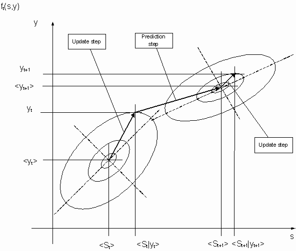
The Kalman Filter is used to predict the inner state s for a sequence of observations y based on the maximum likelihood approach.
Both s and y are disturbed through white gaussian noise. We now assume that the joint likelihood of s and y can be modeled by a gaussian distribution.
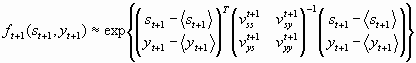
Gaussian Distribution
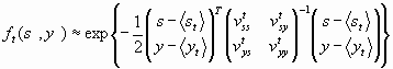
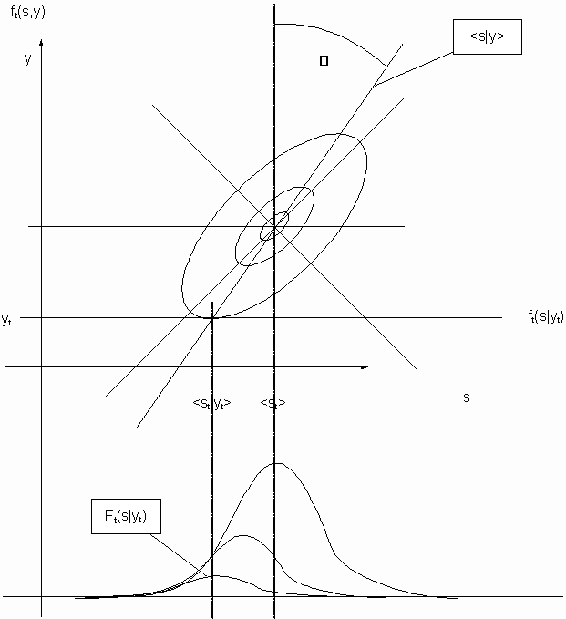
The likelihood that the system is at time t in a specific state is described by a probability density distribution ft(s,y). Now we assume that the distribution ft(s,y) is a multivariate gaussian distribution.
„ st… expected mean value for s assuming the distribution ft(s,y)
„ yt… expected mean value for y assuming the distribution ft(s,y)
vtss expected mean value for „ st st… assuming the distribution ft(s,y)
vtyy expected mean value for „ yt yt… assuming the distribution ft(s,y)
vtsy expected mean value for „ st yt… assuming the distribution ft(s,y)
vtys expected mean value for „ yt st… assuming the distribution ft(s,y)
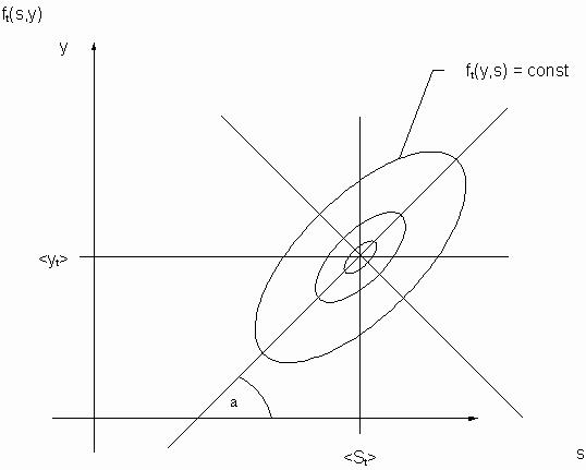
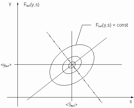
The two dimensional case ft(s,y) = const delivers ellipses as depicted in the figure. We get ellipsoides for the three dimensional case.
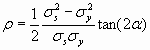
The covariance
![]() can be represented by a product of the standard deviations s
s and s
y weighted by the correlation r
. The correlation itself is a function of the angle a
in order to close the gap between the graphical representation and the common representation of the distribution density function f(s,y).
can be represented by a product of the standard deviations s
s and s
y weighted by the correlation r
. The correlation itself is a function of the angle a
in order to close the gap between the graphical representation and the common representation of the distribution density function f(s,y).
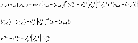
Update step
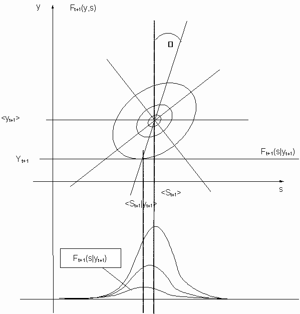
This step delivers the mean and variance for the most likely distribution of s based on a measured y which represents the update for the most likely mean of yt. The distribution ft(s,y) can be reduced to the conditional distribution ft(s|y).assuming that y is known.
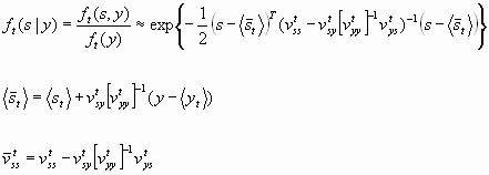
The advantage of the conditional distribution is that it requires less computational effort. However, its derivation is not trivial.
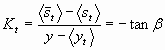
The factor K denotes the Kalman Gain because it determines the influence of the measured value y onto the predicted inner state s.
![]()
The Kalman Gain is related to the angle b in the graphical represenation by the following equation:
Prediction Step
This step delivers the prediction for t+1 with respect to state st+1.

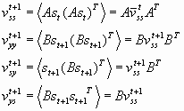
Update Step with Aposteriori Estimate
Algorithm
In order to setup the procedure, firstly a starting value for y,s together with a distribution is assumed. A first measure value of y is used to get the most likely value for s. Based on this update for s, its value is estimated for t+1 employing the transfer function of the system. In addition also the variance is predicted leading to a predicted distribution. This process of updates using measured values and predictions using the transfer function can be repeated iteratively.